Principal Component Analysis (PCA)

Tutorial

Author

Orlando Sabogal-Cardona

Published

May 13, 2024

#Libraries and data

library(tidyverse)

── Attaching core tidyverse packages ──────────────────────── tidyverse 2.0.0 ──
✔ dplyr     1.1.3     ✔ readr     2.1.4
✔ forcats   1.0.0     ✔ stringr   1.5.1
✔ ggplot2   3.4.4     ✔ tibble    3.2.1
✔ lubridate 1.9.3     ✔ tidyr     1.3.0
✔ purrr     1.0.2     
── Conflicts ────────────────────────────────────────── tidyverse_conflicts() ──
✖ dplyr::filter() masks stats::filter()
✖ dplyr::lag()    masks stats::lag()
ℹ Use the conflicted package (<http://conflicted.r-lib.org/>) to force all conflicts to become errors

library(magrittr)


Attaching package: 'magrittr'

The following object is masked from 'package:purrr':

    set_names

The following object is masked from 'package:tidyr':

    extract

library(factoextra)

Warning: package 'factoextra' was built under R version 4.3.3

Welcome! Want to learn more? See two factoextra-related books at https://goo.gl/ve3WBa

library(psych)

Warning: package 'psych' was built under R version 4.3.3


Attaching package: 'psych'

The following objects are masked from 'package:ggplot2':

    %+%, alpha

First example

Iris data

names(iris)

[1] "Sepal.Length" "Sepal.Width"  "Petal.Length" "Petal.Width"  "Species"

MyData <- iris %>% select(-Species)

By hand

summary(MyData)

  Sepal.Length    Sepal.Width     Petal.Length    Petal.Width   
 Min.   :4.300   Min.   :2.000   Min.   :1.000   Min.   :0.100  
 1st Qu.:5.100   1st Qu.:2.800   1st Qu.:1.600   1st Qu.:0.300  
 Median :5.800   Median :3.000   Median :4.350   Median :1.300  
 Mean   :5.843   Mean   :3.057   Mean   :3.758   Mean   :1.199  
 3rd Qu.:6.400   3rd Qu.:3.300   3rd Qu.:5.100   3rd Qu.:1.800  
 Max.   :7.900   Max.   :4.400   Max.   :6.900   Max.   :2.500

MyData_scaled <- scale(MyData)
head(MyData_scaled)

     Sepal.Length Sepal.Width Petal.Length Petal.Width
[1,]   -0.8976739  1.01560199    -1.335752   -1.311052
[2,]   -1.1392005 -0.13153881    -1.335752   -1.311052
[3,]   -1.3807271  0.32731751    -1.392399   -1.311052
[4,]   -1.5014904  0.09788935    -1.279104   -1.311052
[5,]   -1.0184372  1.24503015    -1.335752   -1.311052
[6,]   -0.5353840  1.93331463    -1.165809   -1.048667

Temp <- (MyData$Sepal.Length - mean(MyData$Sepal.Length))/sd(MyData$Sepal.Length)
head(Temp)

[1] -0.8976739 -1.1392005 -1.3807271 -1.5014904 -1.0184372 -0.5353840

# Compute the covariance matrix
cov_matrix <- cov(MyData_scaled)
cov_matrix

             Sepal.Length Sepal.Width Petal.Length Petal.Width
Sepal.Length    1.0000000  -0.1175698    0.8717538   0.8179411
Sepal.Width    -0.1175698   1.0000000   -0.4284401  -0.3661259
Petal.Length    0.8717538  -0.4284401    1.0000000   0.9628654
Petal.Width     0.8179411  -0.3661259    0.9628654   1.0000000

# Eigen decomposition
eigen_results <- eigen(cov_matrix)

eigen_results$values

[1] 2.91849782 0.91403047 0.14675688 0.02071484

eigen_results$vectors

           [,1]        [,2]       [,3]       [,4]
[1,]  0.5210659 -0.37741762  0.7195664  0.2612863
[2,] -0.2693474 -0.92329566 -0.2443818 -0.1235096
[3,]  0.5804131 -0.02449161 -0.1421264 -0.8014492
[4,]  0.5648565 -0.06694199 -0.6342727  0.5235971

# Compute the PCA scores
scores <- MyData_scaled %*% eigen_results$vectors
head(scores)

          [,1]       [,2]        [,3]         [,4]
[1,] -2.257141 -0.4784238  0.12727962  0.024087508
[2,] -2.074013  0.6718827  0.23382552  0.102662845
[3,] -2.356335  0.3407664 -0.04405390  0.028282305
[4,] -2.291707  0.5953999 -0.09098530 -0.065735340
[5,] -2.381863 -0.6446757 -0.01568565 -0.035802870
[6,] -2.068701 -1.4842053 -0.02687825  0.006586116

# Eigenvalues and explained variance
eigenvalues <- eigen_results$values
var_explained <- eigenvalues / sum(eigenvalues) * 100  
pca_df <- data.frame(PC = 1:length(eigenvalues), Variance = var_explained)
pca_df$Cum <- cumsum(pca_df$Variance)

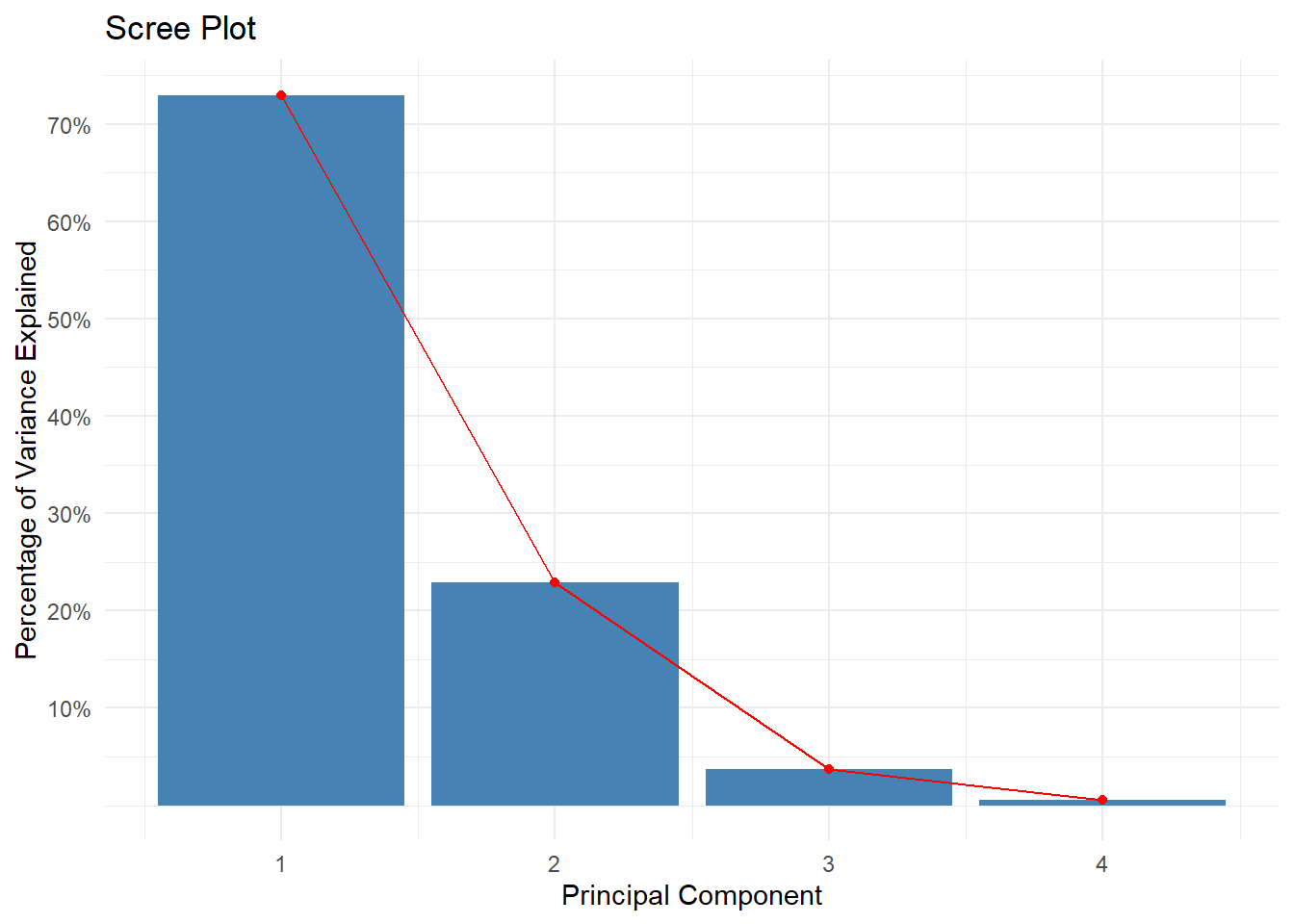
# Create the scree plot
ggplot(pca_df, aes(x = PC, y = Variance)) +
  geom_bar(stat = "identity", fill = "steelblue") +
  geom_line(aes(group = 1), color = "red") +
  geom_point(color = "red") + 
  scale_y_continuous(breaks = c(10, 20, 30, 40, 50, 60, 70),
                     labels = c("10%","20%", "30%", "40%", "50%", "60%", "70%")) +
labs(title = "Scree Plot", 
       x = "Principal Component", 
       y = "Percentage of Variance Explained") +
  theme_minimal()

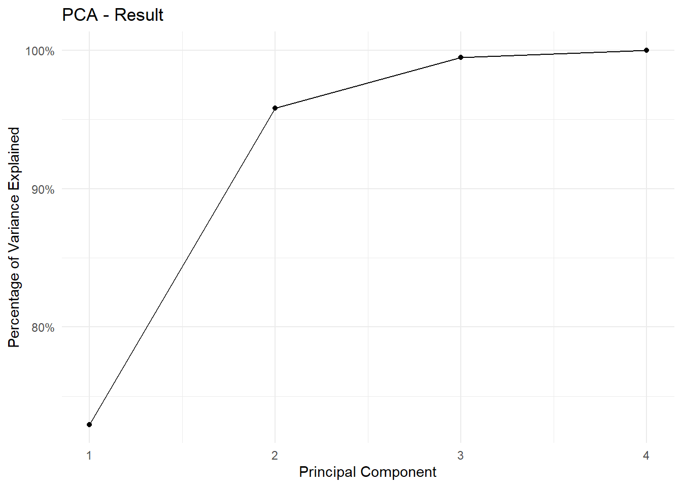
ggplot(data = pca_df, aes(x = PC, y = Cum)) +
  geom_point() +
  geom_line() +
  scale_y_continuous(breaks = c(80, 90, 100),
                     labels = c("80%", "90%", "100%")) +
  labs(title = "PCA - Result", 
       x = "Principal Component", 
       y = "Percentage of Variance Explained") +
  theme_minimal()

scores <- as.data.frame(scores)
names(scores) <- c("PC1", "PC2", "PC3", "PC4")
head(scores)

        PC1        PC2         PC3          PC4
1 -2.257141 -0.4784238  0.12727962  0.024087508
2 -2.074013  0.6718827  0.23382552  0.102662845
3 -2.356335  0.3407664 -0.04405390  0.028282305
4 -2.291707  0.5953999 -0.09098530 -0.065735340
5 -2.381863 -0.6446757 -0.01568565 -0.035802870
6 -2.068701 -1.4842053 -0.02687825  0.006586116

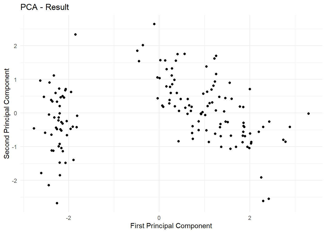
ggplot(data = scores) +
  geom_point(aes(x = PC1, y = PC2)) +
  labs(title = "PCA - Result", 
       x = "First Principal Component", 
       y = "Second Principal Component") +
  theme_minimal()

prcomp

prcomp (scale = FALSE)

MyFirst_PCA <- prcomp(MyData)

MyFirst_PCA

Standard deviations (1, .., p=4):
[1] 2.0562689 0.4926162 0.2796596 0.1543862

Rotation (n x k) = (4 x 4):
                     PC1         PC2         PC3        PC4
Sepal.Length  0.36138659 -0.65658877  0.58202985  0.3154872
Sepal.Width  -0.08452251 -0.73016143 -0.59791083 -0.3197231
Petal.Length  0.85667061  0.17337266 -0.07623608 -0.4798390
Petal.Width   0.35828920  0.07548102 -0.54583143  0.7536574

str(MyFirst_PCA)

List of 5
 $ sdev    : num [1:4] 2.056 0.493 0.28 0.154
 $ rotation: num [1:4, 1:4] 0.3614 -0.0845 0.8567 0.3583 -0.6566 ...
  ..- attr(*, "dimnames")=List of 2
  .. ..$ : chr [1:4] "Sepal.Length" "Sepal.Width" "Petal.Length" "Petal.Width"
  .. ..$ : chr [1:4] "PC1" "PC2" "PC3" "PC4"
 $ center  : Named num [1:4] 5.84 3.06 3.76 1.2
  ..- attr(*, "names")= chr [1:4] "Sepal.Length" "Sepal.Width" "Petal.Length" "Petal.Width"
 $ scale   : logi FALSE
 $ x       : num [1:150, 1:4] -2.68 -2.71 -2.89 -2.75 -2.73 ...
  ..- attr(*, "dimnames")=List of 2
  .. ..$ : NULL
  .. ..$ : chr [1:4] "PC1" "PC2" "PC3" "PC4"
 - attr(*, "class")= chr "prcomp"

$rotation is the matrix of the principal component loadings (eigenvectors). Each column of rotation contains coefficients for one principal component.

MyFirst_PCA$rotation

                     PC1         PC2         PC3        PC4
Sepal.Length  0.36138659 -0.65658877  0.58202985  0.3154872
Sepal.Width  -0.08452251 -0.73016143 -0.59791083 -0.3197231
Petal.Length  0.85667061  0.17337266 -0.07623608 -0.4798390
Petal.Width   0.35828920  0.07548102 -0.54583143  0.7536574

The eigenvalues are a bit tricky. In $sdev you will find the standard deviation of each principal component. It provides a measure of the amount of variation captured by each component. Remember that the igenvalues are associated with the variance of the components. Therefore, you only need to ^2

MyFirst_PCA$sdev

[1] 2.0562689 0.4926162 0.2796596 0.1543862

MyFirst_PCA$sdev^2

[1] 4.22824171 0.24267075 0.07820950 0.02383509

MyFirst_PCA$sdev^2/sum(MyFirst_PCA$sdev^2)

[1] 0.924618723 0.053066483 0.017102610 0.005212184

summary(MyFirst_PCA)

Importance of components:
                          PC1     PC2    PC3     PC4
Standard deviation     2.0563 0.49262 0.2797 0.15439
Proportion of Variance 0.9246 0.05307 0.0171 0.00521
Cumulative Proportion  0.9246 0.97769 0.9948 1.00000

The “scores” of the components:

MyFirst_PCA$x %>% head()

           PC1        PC2         PC3          PC4
[1,] -2.684126 -0.3193972  0.02791483  0.002262437
[2,] -2.714142  0.1770012  0.21046427  0.099026550
[3,] -2.888991  0.1449494 -0.01790026  0.019968390
[4,] -2.745343  0.3182990 -0.03155937 -0.075575817
[5,] -2.728717 -0.3267545 -0.09007924 -0.061258593
[6,] -2.280860 -0.7413304 -0.16867766 -0.024200858

prcomp (scale = TRUE)

MyFirst_PCA <- prcomp(MyData, scale = TRUE)

MyFirst_PCA

Standard deviations (1, .., p=4):
[1] 1.7083611 0.9560494 0.3830886 0.1439265

Rotation (n x k) = (4 x 4):
                    PC1         PC2        PC3        PC4
Sepal.Length  0.5210659 -0.37741762  0.7195664  0.2612863
Sepal.Width  -0.2693474 -0.92329566 -0.2443818 -0.1235096
Petal.Length  0.5804131 -0.02449161 -0.1421264 -0.8014492
Petal.Width   0.5648565 -0.06694199 -0.6342727  0.5235971

MyFirst_PCA$rotation

                    PC1         PC2        PC3        PC4
Sepal.Length  0.5210659 -0.37741762  0.7195664  0.2612863
Sepal.Width  -0.2693474 -0.92329566 -0.2443818 -0.1235096
Petal.Length  0.5804131 -0.02449161 -0.1421264 -0.8014492
Petal.Width   0.5648565 -0.06694199 -0.6342727  0.5235971

summary(MyFirst_PCA)

Importance of components:
                          PC1    PC2     PC3     PC4
Standard deviation     1.7084 0.9560 0.38309 0.14393
Proportion of Variance 0.7296 0.2285 0.03669 0.00518
Cumulative Proportion  0.7296 0.9581 0.99482 1.00000

princomp

PCA_Results <- princomp(MyData, cor = TRUE, scores = TRUE)

PCA_Results

Call:
princomp(x = MyData, cor = TRUE, scores = TRUE)

Standard deviations:
   Comp.1    Comp.2    Comp.3    Comp.4 
1.7083611 0.9560494 0.3830886 0.1439265 

 4  variables and  150 observations.

summary(PCA_Results)

Importance of components:
                          Comp.1    Comp.2     Comp.3      Comp.4
Standard deviation     1.7083611 0.9560494 0.38308860 0.143926497
Proportion of Variance 0.7296245 0.2285076 0.03668922 0.005178709
Cumulative Proportion  0.7296245 0.9581321 0.99482129 1.000000000

str(PCA_Results)

List of 7
 $ sdev    : Named num [1:4] 1.708 0.956 0.383 0.144
  ..- attr(*, "names")= chr [1:4] "Comp.1" "Comp.2" "Comp.3" "Comp.4"
 $ loadings: 'loadings' num [1:4, 1:4] 0.521 -0.269 0.58 0.565 0.377 ...
  ..- attr(*, "dimnames")=List of 2
  .. ..$ : chr [1:4] "Sepal.Length" "Sepal.Width" "Petal.Length" "Petal.Width"
  .. ..$ : chr [1:4] "Comp.1" "Comp.2" "Comp.3" "Comp.4"
 $ center  : Named num [1:4] 5.84 3.06 3.76 1.2
  ..- attr(*, "names")= chr [1:4] "Sepal.Length" "Sepal.Width" "Petal.Length" "Petal.Width"
 $ scale   : Named num [1:4] 0.825 0.434 1.759 0.76
  ..- attr(*, "names")= chr [1:4] "Sepal.Length" "Sepal.Width" "Petal.Length" "Petal.Width"
 $ n.obs   : int 150
 $ scores  : num [1:150, 1:4] -2.26 -2.08 -2.36 -2.3 -2.39 ...
  ..- attr(*, "dimnames")=List of 2
  .. ..$ : NULL
  .. ..$ : chr [1:4] "Comp.1" "Comp.2" "Comp.3" "Comp.4"
 $ call    : language princomp(x = MyData, cor = TRUE, scores = TRUE)
 - attr(*, "class")= chr "princomp"

PCA_Results$loadings


Loadings:
             Comp.1 Comp.2 Comp.3 Comp.4
Sepal.Length  0.521  0.377  0.720  0.261
Sepal.Width  -0.269  0.923 -0.244 -0.124
Petal.Length  0.580        -0.142 -0.801
Petal.Width   0.565        -0.634  0.524

               Comp.1 Comp.2 Comp.3 Comp.4
SS loadings      1.00   1.00   1.00   1.00
Proportion Var   0.25   0.25   0.25   0.25
Cumulative Var   0.25   0.50   0.75   1.00

PCA_Results$scores %>% head()

        Comp.1     Comp.2      Comp.3      Comp.4
[1,] -2.264703  0.4800266  0.12770602  0.02416820
[2,] -2.080961 -0.6741336  0.23460885  0.10300677
[3,] -2.364229 -0.3419080 -0.04420148  0.02837705
[4,] -2.299384 -0.5973945 -0.09129011 -0.06595556
[5,] -2.389842  0.6468354 -0.01573820 -0.03592281
[6,] -2.075631  1.4891775 -0.02696829  0.00660818

prcomp vs princomp

The prcomp() function utilizes something calles Spectral Value Decomposition SVD. The pincomp() function utilizes Spectra Decomposition.

factoextra

MyFirst_PCA <- prcomp(MyData, scale = TRUE)

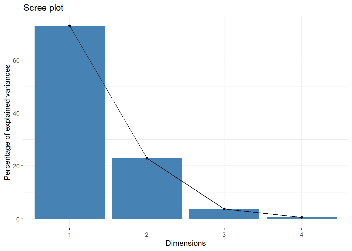
fviz_eig(MyFirst_PCA)

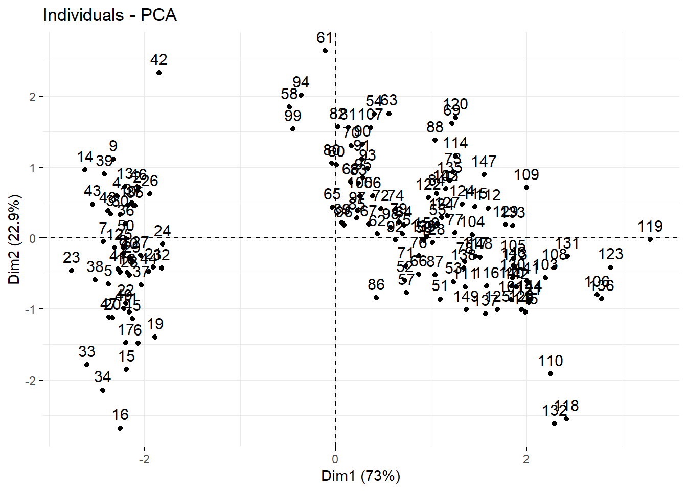
fviz_pca_ind(MyFirst_PCA)

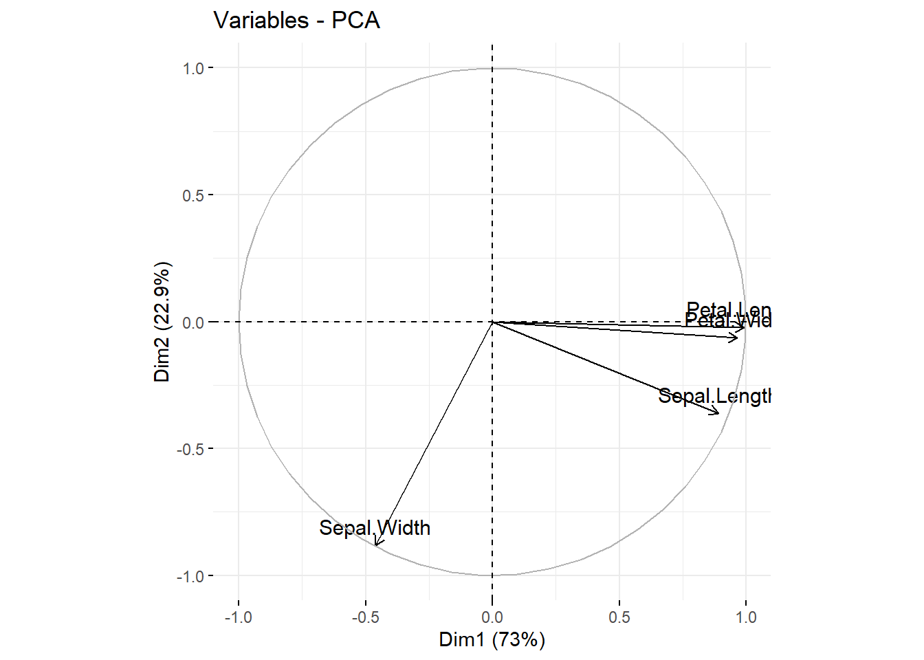
fviz_pca_var(MyFirst_PCA)

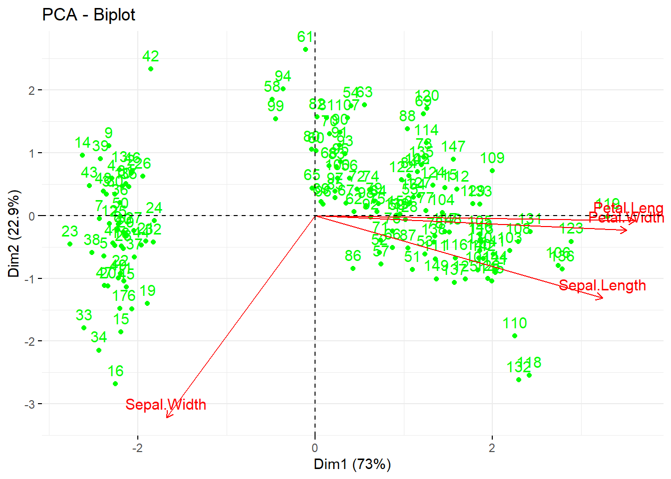
fviz_pca_biplot(MyFirst_PCA,
                col.var = "red", 
                col.ind = "green")

With psych

I personally see the “principal() function from the psych library as a way to bridge gaps between PCA and EFA. EFA is the next big topic we will disccuss.

But as of now, all you need to know is that the concepts of factor rotation and residual correlations are not common in PCA.

PCA_psych <- principal(MyData, 
                       nfactors = 4, # why?
                       residuals = FALSE, # this is the default
                       rotate="varimax") # also the defauls

PCA_psych

Principal Components Analysis
Call: principal(r = MyData, nfactors = 4, residuals = FALSE, rotate = "varimax")
Standardized loadings (pattern matrix) based upon correlation matrix
               RC1   RC3   RC2   RC4 h2       u2 com
Sepal.Length  0.53  0.85  0.00  0.00  1  1.1e-16 1.7
Sepal.Width  -0.17 -0.04  0.98 -0.01  1  4.4e-16 1.1
Petal.Length  0.78  0.54 -0.28  0.14  1 -4.4e-16 2.2
Petal.Width   0.89  0.41 -0.20 -0.06  1  0.0e+00 1.5

                       RC1  RC3  RC2  RC4
SS loadings           1.71 1.18 1.09 0.02
Proportion Var        0.43 0.30 0.27 0.01
Cumulative Var        0.43 0.72 0.99 1.00
Proportion Explained  0.43 0.30 0.27 0.01
Cumulative Proportion 0.43 0.72 0.99 1.00

Mean item complexity =  1.6
Test of the hypothesis that 4 components are sufficient.

The root mean square of the residuals (RMSR) is  0 
 with the empirical chi square  0  with prob <  NA 

Fit based upon off diagonal values = 1

PCA_psych$values

[1] 2.91849782 0.91403047 0.14675688 0.02071484

Second example

head(decathlon2)

          X100m Long.jump Shot.put High.jump X400m X110m.hurdle Discus
SEBRLE    11.04      7.58    14.83      2.07 49.81        14.69  43.75
CLAY      10.76      7.40    14.26      1.86 49.37        14.05  50.72
BERNARD   11.02      7.23    14.25      1.92 48.93        14.99  40.87
YURKOV    11.34      7.09    15.19      2.10 50.42        15.31  46.26
ZSIVOCZKY 11.13      7.30    13.48      2.01 48.62        14.17  45.67
McMULLEN  10.83      7.31    13.76      2.13 49.91        14.38  44.41
          Pole.vault Javeline X1500m Rank Points Competition
SEBRLE          5.02    63.19  291.7    1   8217    Decastar
CLAY            4.92    60.15  301.5    2   8122    Decastar
BERNARD         5.32    62.77  280.1    4   8067    Decastar
YURKOV          4.72    63.44  276.4    5   8036    Decastar
ZSIVOCZKY       4.42    55.37  268.0    7   8004    Decastar
McMULLEN        4.42    56.37  285.1    8   7995    Decastar

Your turn!